California Housing Price Prediction

7 minute read

DESCRIPTION

Background of Problem Statement :

The US Census Bureau has published California Census Data which has 10 types of metrics such as the population, median income, median housing price, and so on for each block group in California. The dataset also serves as an input for project scoping and tries to specify the functional and nonfunctional requirements for it.

Problem Objective :

The project aims at building a model of housing prices to predict median house values in California using the provided dataset. This model should learn from the data and be able to predict the median housing price in any district, given all the other metrics.

Districts or block groups are the smallest geographical units for which the US Census Bureau publishes sample data (a block group typically has a population of 600 to 3,000 people). There are 20,640 districts in the project dataset.

Domain: Finance and Housing

Analysis Tasks to be performed:

Build a model of housing prices to predict median house values in California using the provided dataset.
Train the model to learn from the data to predict the median housing price in any district, given all the other metrics.
Predict housing prices based on median_income and plot the regression chart for it.

#Import Necessary Libraries:
import pandas as pd
import numpy as np

from sklearn.preprocessing import LabelEncoder,StandardScaler
from sklearn.linear_model import LinearRegression,Ridge,Lasso,ElasticNet
from sklearn.tree import DecisionTreeRegressor
import statsmodels.formula.api as smf

from sklearn.metrics import mean_squared_error,r2_score
from math import sqrt

import seaborn as sns
import matplotlib.pyplot as plt
%matplotlib inline

import warnings
warnings.filterwarnings('ignore')

from matplotlib.axes._axes import _log as matplotlib_axes_logger
matplotlib_axes_logger.setLevel('ERROR')

1. Load Data

Read the “housing.csv” file from the folder into the program.
Print first few rows of this data.

df_house=pd.read_excel("Dataset/1553768847_housing.xlsx")

df_house.head()

	longitude	latitude	housing_median_age	total_rooms	total_bedrooms	population	households	median_income	ocean_proximity	median_house_value
0	-122.23	37.88	41	880	129.0	322	126	8.3252	NEAR BAY	452600
1	-122.22	37.86	21	7099	1106.0	2401	1138	8.3014	NEAR BAY	358500
2	-122.24	37.85	52	1467	190.0	496	177	7.2574	NEAR BAY	352100
3	-122.25	37.85	52	1274	235.0	558	219	5.6431	NEAR BAY	341300
4	-122.25	37.85	52	1627	280.0	565	259	3.8462	NEAR BAY	342200

import math
print(math.log(452600))

13.022764012181574

df_house.columns

Index(['longitude', 'latitude', 'housing_median_age', 'total_rooms',
       'total_bedrooms', 'population', 'households', 'median_income',
       'ocean_proximity', 'median_house_value'],
      dtype='object')

2. Handle missing values :

Fill the missing values with the mean of the respective column.

df_house.isnull().sum()

longitude               0
latitude                0
housing_median_age      0
total_rooms             0
total_bedrooms        207
population              0
households              0
median_income           0
ocean_proximity         0
median_house_value      0
dtype: int64

We see that there are 207 null values in Column total_bedrooms. We replace the null values with the mean and check for nulls again.

df_house.total_bedrooms=df_house.total_bedrooms.fillna(df_house.total_bedrooms.mean())
df_house.isnull().sum()

longitude             0
latitude              0
housing_median_age    0
total_rooms           0
total_bedrooms        0
population            0
households            0
median_income         0
ocean_proximity       0
median_house_value    0
dtype: int64

3. Encode categorical data :

Convert categorical column in the dataset to numerical data.

le = LabelEncoder()
df_house['ocean_proximity']=le.fit_transform(df_house['ocean_proximity'])

4. Standardize data :

Standardize training and test datasets.

# Get column names first
names = df_house.columns
# Create the Scaler object
scaler = StandardScaler()
# Fit your data on the scaler object
scaled_df = scaler.fit_transform(df_house)
scaled_df = pd.DataFrame(scaled_df, columns=names)
scaled_df.head()

	longitude	latitude	housing_median_age	total_rooms	total_bedrooms	population	households	median_income	ocean_proximity	median_house_value
0	-1.327835	1.052548	0.982143	-0.804819	-0.975228	-0.974429	-0.977033	2.344766	1.291089	2.129631
1	-1.322844	1.043185	-0.607019	2.045890	1.355088	0.861439	1.669961	2.332238	1.291089	1.314156
2	-1.332827	1.038503	1.856182	-0.535746	-0.829732	-0.820777	-0.843637	1.782699	1.291089	1.258693
3	-1.337818	1.038503	1.856182	-0.624215	-0.722399	-0.766028	-0.733781	0.932968	1.291089	1.165100
4	-1.337818	1.038503	1.856182	-0.462404	-0.615066	-0.759847	-0.629157	-0.012881	1.291089	1.172900

5. visualize relationship between features and target

Check for Linearity

#plot graphs
fig,axs=plt.subplots(1,3,sharey=True)
scaled_df.plot(kind='scatter',x='longitude',y='median_house_value',ax=axs[0],figsize=(16,8))
scaled_df.plot(kind='scatter',x='latitude',y='median_house_value',ax=axs[1],figsize=(16,8))
scaled_df.plot(kind='scatter',x='housing_median_age',y='median_house_value',ax=axs[2],figsize=(16,8))

#plot graphs
fig,axs=plt.subplots(1,3,sharey=True)
scaled_df.plot(kind='scatter',x='total_rooms',y='median_house_value',ax=axs[0],figsize=(16,8))
scaled_df.plot(kind='scatter',x='total_bedrooms',y='median_house_value',ax=axs[1],figsize=(16,8))
scaled_df.plot(kind='scatter',x='population',y='median_house_value',ax=axs[2],figsize=(16,8))

#plot graphs
fig,axs=plt.subplots(1,3,sharey=True)
scaled_df.plot(kind='scatter',x='households',y='median_house_value',ax=axs[0],figsize=(16,8))
scaled_df.plot(kind='scatter',x='median_income',y='median_house_value',ax=axs[1],figsize=(16,8))
scaled_df.plot(kind='scatter',x='ocean_proximity',y='median_house_value',ax=axs[2],figsize=(16,8))

<matplotlib.axes._subplots.AxesSubplot at 0x288205cf588>

png

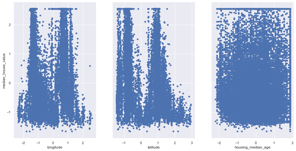
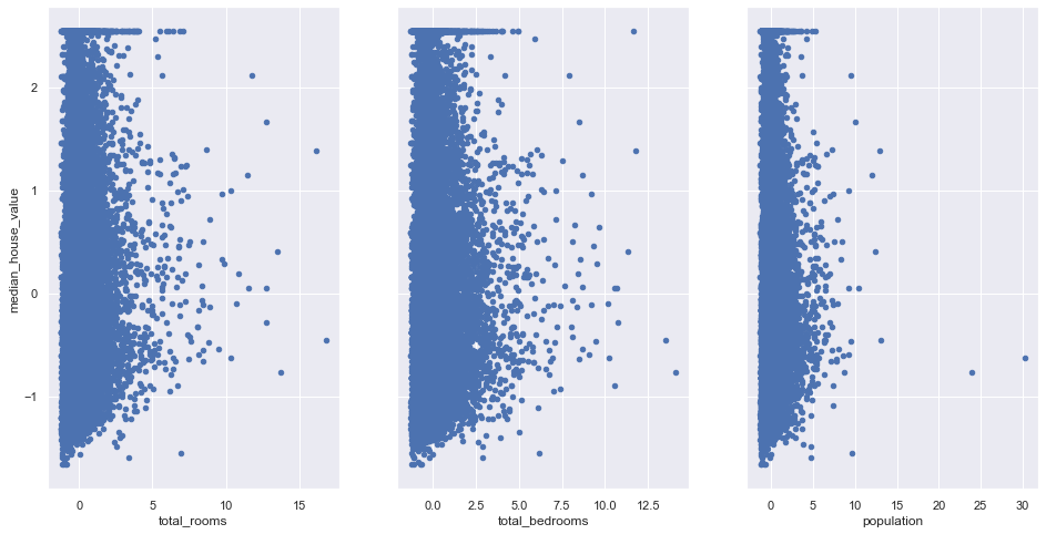
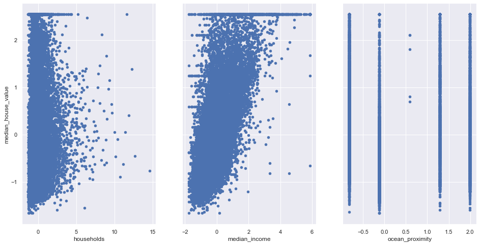
Insight:

The above graphs shows that only median_income and median_house_value has a linear relationship.

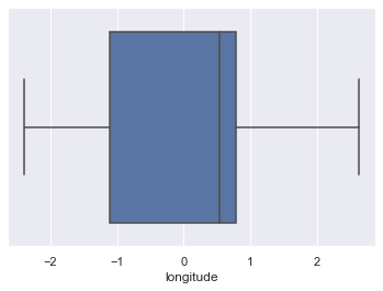
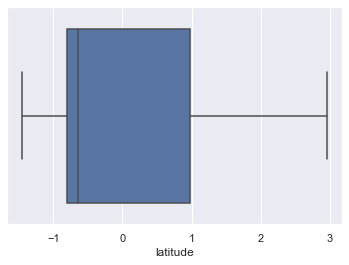
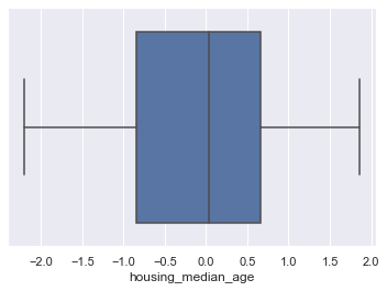
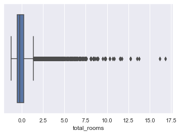
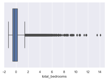
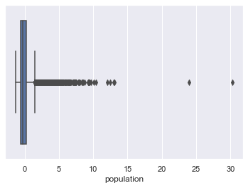
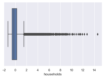
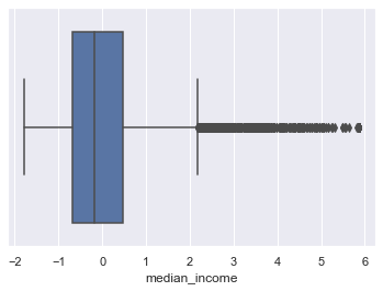
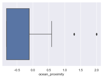
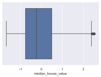
Check for Outliers:

for column in scaled_df:
    plt.figure()
    sns.boxplot(x=scaled_df[column])

png

6. Extract X and Y data :

Extract input (X) and output (Y) data from the dataset.

X_Features=['longitude', 'latitude', 'housing_median_age', 'total_rooms',
       'total_bedrooms', 'population', 'households', 'median_income',
       'ocean_proximity']
X=scaled_df[X_Features]
Y=scaled_df['median_house_value']

print(type(X))
print(type(Y))

<class 'pandas.core.frame.DataFrame'>
<class 'pandas.core.series.Series'>

print(df_house.shape)
print(X.shape)
print(Y.shape)

(20640, 10)
(20640, 9)
(20640,)

7. Split the dataset :

Split the data into 80% training dataset and 20% test dataset.

from sklearn.model_selection import train_test_split
x_train,x_test,y_train,y_test=train_test_split(X,Y,test_size=0.2,random_state=1)

print (x_train.shape, y_train.shape)
print (x_test.shape, y_test.shape)

(16512, 9) (16512,)
(4128, 9) (4128,)

8. Apply Various Algorithms:

Linear Regression
Decision Tree Regression
Random Forest Regression (Ensemble Learning)
Lasso
Ridge
Elastic Net

Perform Linear Regression :

Perform Linear Regression on training data.
Predict output for test dataset using the fitted model.
Print root mean squared error (RMSE) from Linear Regression.

linreg=LinearRegression()
linreg.fit(x_train,y_train)

LinearRegression(copy_X=True, fit_intercept=True, n_jobs=None, normalize=False)

y_predict = linreg.predict(x_test)

print(sqrt(mean_squared_error(y_test,y_predict)))
print((r2_score(y_test,y_predict)))

0.6056598120301221
0.6276223517950296

Perform Decision Tree Regression :

Perform Decision Tree Regression on training data.
Predict output for test dataset using the fitted model.
Print root mean squared error from Decision Tree Regression.

dtreg=DecisionTreeRegressor()
dtreg.fit(x_train,y_train)

DecisionTreeRegressor(criterion='mse', max_depth=None, max_features=None,
                      max_leaf_nodes=None, min_impurity_decrease=0.0,
                      min_impurity_split=None, min_samples_leaf=1,
                      min_samples_split=2, min_weight_fraction_leaf=0.0,
                      presort=False, random_state=None, splitter='best')

y_predict = dtreg.predict(x_test)
print(sqrt(mean_squared_error(y_test,y_predict)))
print((r2_score(y_test,y_predict)))

0.5912422593872186
0.6451400183074161

Perform Random Forest Regression :

Perform Random Forest Regression on training data.
Predict output for test dataset using the fitted model.
Print RMSE (root mean squared error) from Random Forest Regression.

rfreg=RandomForestRegressor()
rfreg.fit(x_train,y_train)

RandomForestRegressor(bootstrap=True, criterion='mse', max_depth=None,
                      max_features='auto', max_leaf_nodes=None,
                      min_impurity_decrease=0.0, min_impurity_split=None,
                      min_samples_leaf=1, min_samples_split=2,
                      min_weight_fraction_leaf=0.0, n_estimators=10,
                      n_jobs=None, oob_score=False, random_state=None,
                      verbose=0, warm_start=False)

y_predict = rfreg.predict(x_test)
print(sqrt(mean_squared_error(y_test,y_predict)))
print((r2_score(y_test,y_predict)))

0.4478028477744602
0.7964365549457926

Perform Lasso Regression (determine which variables should be retained in the model):

Perform Lasso Regression on training data.
Predict output for test dataset using the fitted model.
Print RMSE (root mean squared error) from Lasso Regression.

lassoreg=Lasso(alpha=0.001,normalize=True)
lassoreg.fit(x_train,y_train)
print(sqrt(mean_squared_error(y_test,lassoreg.predict(x_test))))
print('R2 Value/Coefficient of determination:{}'.format(lassoreg.score(x_test,y_test)))

0.7193140967070711
R2 Value/Coefficient of determination:0.4747534206169959

Perform Ridge Regression (addresses multicollinearity issues) :

Perform Ridge Regression on training data.
Predict output for test dataset using the fitted model.
Print RMSE (root mean squared error) from Ridge Regression.

ridgereg=Ridge(alpha=0.001,normalize=True)
ridgereg.fit(x_train,y_train)
print(sqrt(mean_squared_error(y_test,ridgereg.predict(x_test))))
print('R2 Value/Coefficient of determination:{}'.format(ridgereg.score(x_test,y_test)))

0.6056048844852343
R2 Value/Coefficient of determination:0.6276898909055972

Perform ElasticNet Regression :

Perform ElasticNet Regression on training data.
Predict output for test dataset using the fitted model.
Print RMSE (root mean squared error) from ElasticNet Regression.

from sklearn.linear_model import ElasticNet
elasticreg=ElasticNet(alpha=0.001,normalize=True)
elasticreg.fit(x_train,y_train)
print(sqrt(mean_squared_error(y_test,elasticreg.predict(x_test))))
print('R2 Value/Coefficient of determination:{}'.format(elasticreg.score(x_test,y_test)))

0.944358169398106
R2 Value/Coefficient of determination:0.09468529806704551

Hypothesis testing and P values:

lm=smf.ols(formula='median_house_value ~ longitude+latitude+housing_median_age+total_rooms+total_bedrooms+population+households+median_income+ocean_proximity',data=scaled_df).fit()

lm.summary()

OLS Regression Results
Dep. Variable:	median_house_value	R-squared:	0.636
Model:	OLS	Adj. R-squared:	0.635
Method:	Least Squares	F-statistic:	3999.
Date:	Thu, 10 Oct 2019	Prob (F-statistic):	0.00
Time:	16:09:59	Log-Likelihood:	-18868.
No. Observations:	20640	AIC:	3.776e+04
Df Residuals:	20630	BIC:	3.783e+04
Df Model:	9
Covariance Type:	nonrobust

	coef	std err	t	P>\|t\|	[0.025	0.975]
Intercept	-4.857e-17	0.004	-1.16e-14	1.000	-0.008	0.008
longitude	-0.7393	0.013	-57.263	0.000	-0.765	-0.714
latitude	-0.7858	0.013	-61.664	0.000	-0.811	-0.761
housing_median_age	0.1248	0.005	26.447	0.000	0.116	0.134
total_rooms	-0.1265	0.015	-8.609	0.000	-0.155	-0.098
total_bedrooms	0.2995	0.022	13.630	0.000	0.256	0.343
population	-0.3907	0.011	-36.927	0.000	-0.411	-0.370
households	0.2589	0.022	11.515	0.000	0.215	0.303
median_income	0.6549	0.005	119.287	0.000	0.644	0.666
ocean_proximity	0.0009	0.005	0.190	0.850	-0.008	0.010

Omnibus:	5037.491	Durbin-Watson:	0.965
Prob(Omnibus):	0.000	Jarque-Bera (JB):	18953.000
Skew:	1.184	Prob(JB):	0.00
Kurtosis:	7.054	Cond. No.	14.2

Warnings:
[1] Standard Errors assume that the covariance matrix of the errors is correctly specified.

Perform Linear Regression with one independent variable :

Extract just the median_income column from the independent variables (from X_train and X_test).
Perform Linear Regression to predict housing values based on median_income.
Predict output for test dataset using the fitted model.
Plot the fitted model for training data as well as for test data to check if the fitted model satisfies the test data.

x_train_Income=x_train[['median_income']]
x_test_Income=x_test[['median_income']]

print(x_train_Income.shape)
print(y_train.shape)

(16512, 1)
(16512,)

visualize relationship between features

linreg=LinearRegression()
linreg.fit(x_train_Income,y_train)
y_predict = linreg.predict(x_test_Income)

#print intercept and coefficient of the linear equation
print(linreg.intercept_, linreg.coef_)
print(sqrt(mean_squared_error(y_test,y_predict)))
print((r2_score(y_test,y_predict)))

005623019866893162 [0.69238221]
7212595914243148
47190835934467734

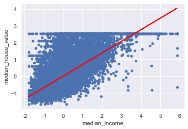
Insight:

Looking at the above values we can say that coefficient: a unit increase in median_income increases the median_house_value by 0.692 unit

#plot least square line
scaled_df.plot(kind='scatter',x='median_income',y='median_house_value')
plt.plot(x_test_Income,y_predict,c='red',linewidth=2)

[<matplotlib.lines.Line2D at 0x28824544240>]

png

Hypothesis testing and P values:

using the null hypothesis lets assume there is no relationship between median_income and median_house_value
Lets test this hypothesis. We shall reject the Null Hypothesis if 95% confidence inderval does not include 0

lm=smf.ols(formula='median_house_value ~ median_income',data=scaled_df).fit()

lm.summary()

OLS Regression Results
Dep. Variable:	median_house_value	R-squared:	0.473
Model:	OLS	Adj. R-squared:	0.473
Method:	Least Squares	F-statistic:	1.856e+04
Date:	Thu, 10 Oct 2019	Prob (F-statistic):	0.00
Time:	16:10:17	Log-Likelihood:	-22668.
No. Observations:	20640	AIC:	4.534e+04
Df Residuals:	20638	BIC:	4.536e+04
Df Model:	1
Covariance Type:	nonrobust

	coef	std err	t	P>\|t\|	[0.025	0.975]
Intercept	-4.857e-17	0.005	-9.62e-15	1.000	-0.010	0.010
median_income	0.6881	0.005	136.223	0.000	0.678	0.698

Omnibus:	4245.795	Durbin-Watson:	0.655
Prob(Omnibus):	0.000	Jarque-Bera (JB):	9273.446
Skew:	1.191	Prob(JB):	0.00
Kurtosis:	5.260	Cond. No.	1.00

Warnings:
[1] Standard Errors assume that the covariance matrix of the errors is correctly specified.

Insight:

The P value is 0.000 indicates strong evidence against the null hypothesis, so you reject the null hypothesis.
 so, there is a strong relationship between median_house_value and median_income

Share on

Twitter Facebook Google+ LinkedIn

Jhimli Bora

California Housing Price Prediction

DESCRIPTION

Background of Problem Statement :

Problem Objective :

Analysis Tasks to be performed:

1. Load Data

2. Handle missing values :

3. Encode categorical data :

4. Standardize data :

5. visualize relationship between features and target

Insight:

6. Extract X and Y data :

7. Split the dataset :

8. Apply Various Algorithms:

Perform Linear Regression :

Perform Decision Tree Regression :

Perform Random Forest Regression :

Perform Lasso Regression (determine which variables should be retained in the model):

Perform Ridge Regression (addresses multicollinearity issues) :

Perform ElasticNet Regression :

Hypothesis testing and P values:

Perform Linear Regression with one independent variable :

Insight:

Hypothesis testing and P values:

Insight:

Share on

You May Also Enjoy

Strength Of High Performance Concrete

Income Qualification