
Income Qualification
DESCRIPTION
Identify the level of income qualification needed for the families in Latin America.
Problem Statement Scenario:
Many social programs have a hard time ensuring that the right people are given enough aid. It’s tricky when a program focuses on the poorest segment of the population. This segment of the population can’t provide the necessary income and expense records to prove that they qualify.
In Latin America, a popular method called Proxy Means Test (PMT) uses an algorithm to verify income qualification. With PMT, agencies use a model that considers a family’s observable household attributes like the material of their walls and ceiling or the assets found in their homes to classify them and predict their level of need.
While this is an improvement, accuracy remains a problem as the region’s population grows and poverty declines.
The Inter-American Development Bank (IDB)believes that new methods beyond traditional econometrics, based on a dataset of Costa Rican household characteristics, might help improve PMT’s performance.
Analysis Tasks to be performed:
- Identify the output variable.
- Understand the type of data.
- Check if there are any biases in your dataset.
- Check whether all members of the house have the same poverty level.
- Check if there is a house without a family head.
- Set poverty level of the members and the head of the house within a family.
- Count how many null values are existing in columns.
- Remove null value rows of the target variable.
- Predict the accuracy using random forest classifier.
- Check the accuracy using random forest with cross validation.
Core Data fields
- Id - a unique identifier for each row.
- Target - the target is an ordinal variable indicating groups of income levels.
1 = extreme poverty 2 = moderate poverty 3 = vulnerable households 4 = non vulnerable households - idhogar - this is a unique identifier for each household. This can be used to create household-wide features, etc. All rows in a given household will have a matching value for this identifier.
- parentesco1 - indicates if this person is the head of the household.
Note: that ONLY the heads of household are used in scoring. All household members are included in train +test data sets, but only heads of households are scored.
Step 1: Understand the Data
1.1 Import necessary Libraries
import numpy as np
import pandas as pd
import matplotlib.pyplot as plt
%matplotlib inline
import seaborn as sns
sns.set()


import warnings
warnings.filterwarnings('ignore')
1.2 Load Data
df_income_train = pd.read_csv("Dataset/train.csv")
df_income_test =  pd.read_csv("Dataset/test.csv")
1.3 Explore Train dataset
View first 5 records of train dataset
df_income_train.head()
| Id | v2a1 | hacdor | rooms | hacapo | v14a | refrig | v18q | v18q1 | r4h1 | ... | SQBescolari | SQBage | SQBhogar_total | SQBedjefe | SQBhogar_nin | SQBovercrowding | SQBdependency | SQBmeaned | agesq | Target | |
|---|---|---|---|---|---|---|---|---|---|---|---|---|---|---|---|---|---|---|---|---|---|
| 0 | ID_279628684 | 190000.0 | 0 | 3 | 0 | 1 | 1 | 0 | NaN | 0 | ... | 100 | 1849 | 1 | 100 | 0 | 1.000000 | 0.0 | 100.0 | 1849 | 4 |
| 1 | ID_f29eb3ddd | 135000.0 | 0 | 4 | 0 | 1 | 1 | 1 | 1.0 | 0 | ... | 144 | 4489 | 1 | 144 | 0 | 1.000000 | 64.0 | 144.0 | 4489 | 4 |
| 2 | ID_68de51c94 | NaN | 0 | 8 | 0 | 1 | 1 | 0 | NaN | 0 | ... | 121 | 8464 | 1 | 0 | 0 | 0.250000 | 64.0 | 121.0 | 8464 | 4 |
| 3 | ID_d671db89c | 180000.0 | 0 | 5 | 0 | 1 | 1 | 1 | 1.0 | 0 | ... | 81 | 289 | 16 | 121 | 4 | 1.777778 | 1.0 | 121.0 | 289 | 4 |
| 4 | ID_d56d6f5f5 | 180000.0 | 0 | 5 | 0 | 1 | 1 | 1 | 1.0 | 0 | ... | 121 | 1369 | 16 | 121 | 4 | 1.777778 | 1.0 | 121.0 | 1369 | 4 |
5 rows × 143 columns
df_income_train.info()
<class 'pandas.core.frame.DataFrame'>
RangeIndex: 9557 entries, 0 to 9556
Columns: 143 entries, Id to Target
dtypes: float64(8), int64(130), object(5)
memory usage: 10.4+ MB
1.4 Explore Test dataset
View first 5 records of test dataset
df_income_test.head()
| Id | v2a1 | hacdor | rooms | hacapo | v14a | refrig | v18q | v18q1 | r4h1 | ... | age | SQBescolari | SQBage | SQBhogar_total | SQBedjefe | SQBhogar_nin | SQBovercrowding | SQBdependency | SQBmeaned | agesq | |
|---|---|---|---|---|---|---|---|---|---|---|---|---|---|---|---|---|---|---|---|---|---|
| 0 | ID_2f6873615 | NaN | 0 | 5 | 0 | 1 | 1 | 0 | NaN | 1 | ... | 4 | 0 | 16 | 9 | 0 | 1 | 2.25 | 0.25 | 272.25 | 16 |
| 1 | ID_1c78846d2 | NaN | 0 | 5 | 0 | 1 | 1 | 0 | NaN | 1 | ... | 41 | 256 | 1681 | 9 | 0 | 1 | 2.25 | 0.25 | 272.25 | 1681 |
| 2 | ID_e5442cf6a | NaN | 0 | 5 | 0 | 1 | 1 | 0 | NaN | 1 | ... | 41 | 289 | 1681 | 9 | 0 | 1 | 2.25 | 0.25 | 272.25 | 1681 |
| 3 | ID_a8db26a79 | NaN | 0 | 14 | 0 | 1 | 1 | 1 | 1.0 | 0 | ... | 59 | 256 | 3481 | 1 | 256 | 0 | 1.00 | 0.00 | 256.00 | 3481 |
| 4 | ID_a62966799 | 175000.0 | 0 | 4 | 0 | 1 | 1 | 1 | 1.0 | 0 | ... | 18 | 121 | 324 | 1 | 0 | 1 | 0.25 | 64.00 | NaN | 324 |
5 rows × 142 columns
df_income_test.info()
<class 'pandas.core.frame.DataFrame'>
RangeIndex: 23856 entries, 0 to 23855
Columns: 142 entries, Id to agesq
dtypes: float64(8), int64(129), object(5)
memory usage: 25.8+ MB
Looking at the train and test dataset we noticed that the following:
Train dataset:
Rows: 9557 entries, 0 to 9556
Columns: 143 entries, Id to Target
Column dtypes: float64(8), int64(130), object(5)
Test dataset:
Rows: 23856 entries, 0 to 23855
Columns: 142 entries, Id to agesq
dtypes: float64(8), int64(129), object(5)
The important piece of information here is that we don’t have ‘Target’ feature in Test Dataset. There are 5 object type, 130(Train set)/ 129 (test set) integer type and 8 float type features. Lets look at those features next.
#List the columns for different datatypes:
print('Integer Type: ')
print(df_income_train.select_dtypes(np.int64).columns)
print('\n')
print('Float Type: ')
print(df_income_train.select_dtypes(np.float64).columns)
print('\n')
print('Object Type: ')
print(df_income_train.select_dtypes(np.object).columns)
Integer Type:
Index(['hacdor', 'rooms', 'hacapo', 'v14a', 'refrig', 'v18q', 'r4h1', 'r4h2',
       'r4h3', 'r4m1',
       ...
       'area1', 'area2', 'age', 'SQBescolari', 'SQBage', 'SQBhogar_total',
       'SQBedjefe', 'SQBhogar_nin', 'agesq', 'Target'],
      dtype='object', length=130)


Float Type:
Index(['v2a1', 'v18q1', 'rez_esc', 'meaneduc', 'overcrowding',
       'SQBovercrowding', 'SQBdependency', 'SQBmeaned'],
      dtype='object')


Object Type:
Index(['Id', 'idhogar', 'dependency', 'edjefe', 'edjefa'], dtype='object')
df_income_train.select_dtypes('int64').head()
| hacdor | rooms | hacapo | v14a | refrig | v18q | r4h1 | r4h2 | r4h3 | r4m1 | ... | area1 | area2 | age | SQBescolari | SQBage | SQBhogar_total | SQBedjefe | SQBhogar_nin | agesq | Target | |
|---|---|---|---|---|---|---|---|---|---|---|---|---|---|---|---|---|---|---|---|---|---|
| 0 | 0 | 3 | 0 | 1 | 1 | 0 | 0 | 1 | 1 | 0 | ... | 1 | 0 | 43 | 100 | 1849 | 1 | 100 | 0 | 1849 | 4 |
| 1 | 0 | 4 | 0 | 1 | 1 | 1 | 0 | 1 | 1 | 0 | ... | 1 | 0 | 67 | 144 | 4489 | 1 | 144 | 0 | 4489 | 4 |
| 2 | 0 | 8 | 0 | 1 | 1 | 0 | 0 | 0 | 0 | 0 | ... | 1 | 0 | 92 | 121 | 8464 | 1 | 0 | 0 | 8464 | 4 |
| 3 | 0 | 5 | 0 | 1 | 1 | 1 | 0 | 2 | 2 | 1 | ... | 1 | 0 | 17 | 81 | 289 | 16 | 121 | 4 | 289 | 4 |
| 4 | 0 | 5 | 0 | 1 | 1 | 1 | 0 | 2 | 2 | 1 | ... | 1 | 0 | 37 | 121 | 1369 | 16 | 121 | 4 | 1369 | 4 |
5 rows × 130 columns
1.5 Find columns with null values
#Find columns with null values
null_counts=df_income_train.select_dtypes('int64').isnull().sum()
null_counts[null_counts > 0]
Series([], dtype: int64)
df_income_train.select_dtypes('float64').head()
| v2a1 | v18q1 | rez_esc | meaneduc | overcrowding | SQBovercrowding | SQBdependency | SQBmeaned | |
|---|---|---|---|---|---|---|---|---|
| 0 | 190000.0 | NaN | NaN | 10.0 | 1.000000 | 1.000000 | 0.0 | 100.0 |
| 1 | 135000.0 | 1.0 | NaN | 12.0 | 1.000000 | 1.000000 | 64.0 | 144.0 |
| 2 | NaN | NaN | NaN | 11.0 | 0.500000 | 0.250000 | 64.0 | 121.0 |
| 3 | 180000.0 | 1.0 | 1.0 | 11.0 | 1.333333 | 1.777778 | 1.0 | 121.0 |
| 4 | 180000.0 | 1.0 | NaN | 11.0 | 1.333333 | 1.777778 | 1.0 | 121.0 |
#Find columns with null values
null_counts=df_income_train.select_dtypes('float64').isnull().sum()
null_counts[null_counts > 0]
v2a1         6860
v18q1        7342
rez_esc      7928
meaneduc        5
SQBmeaned       5
dtype: int64
df_income_train.select_dtypes('object').head()
| Id | idhogar | dependency | edjefe | edjefa | |
|---|---|---|---|---|---|
| 0 | ID_279628684 | 21eb7fcc1 | no | 10 | no |
| 1 | ID_f29eb3ddd | 0e5d7a658 | 8 | 12 | no |
| 2 | ID_68de51c94 | 2c7317ea8 | 8 | no | 11 |
| 3 | ID_d671db89c | 2b58d945f | yes | 11 | no |
| 4 | ID_d56d6f5f5 | 2b58d945f | yes | 11 | no |
#Find columns with null values
null_counts=df_income_train.select_dtypes('object').isnull().sum()
null_counts[null_counts > 0]
Series([], dtype: int64)
Looking at the different types of data and null values for each feature. We found the following: 1. No null values for Integer type features. 2. No null values for float type features. 3. For Object types v2a1 6860 v18q1 7342 rez_esc 7928 meaneduc 5 SQBmeaned 5
We also noticed that object type features dependency, edjefe, edjefa have mixed values.
Lets fix the data for features with null values and features with mixed values
Step 3: Data Cleaning
3.1 Lets fix the column with mixed values.
According to the documentation for these columns:
dependency: Dependency rate, calculated = (number of members of the household younger than 19 or older than 64)/(number of member of household between 19 and 64)
edjefe: years of education of male head of household, based on the interaction of escolari (years of education), head of household and gender, yes=1 and no=0
edjefa: years of education of female head of household, based on the interaction of escolari (years of education), head of household and gender, yes=1 and no=0
For these three variables, it seems “yes” = 1 and “no” = 0. We can correct the variables using a mapping and convert to floats.
mapping={'yes':1,'no':0}

for df in [df_income_train, df_income_test]:
    df['dependency'] =df['dependency'].replace(mapping).astype(np.float64)
    df['edjefe'] =df['edjefe'].replace(mapping).astype(np.float64)
    df['edjefa'] =df['edjefa'].replace(mapping).astype(np.float64)

df_income_train[['dependency','edjefe','edjefa']].describe()
| dependency | edjefe | edjefa | |
|---|---|---|---|
| count | 9557.000000 | 9557.000000 | 9557.000000 |
| mean | 1.149550 | 5.096788 | 2.896830 |
| std | 1.605993 | 5.246513 | 4.612056 |
| min | 0.000000 | 0.000000 | 0.000000 |
| 25% | 0.333333 | 0.000000 | 0.000000 |
| 50% | 0.666667 | 6.000000 | 0.000000 |
| 75% | 1.333333 | 9.000000 | 6.000000 |
| max | 8.000000 | 21.000000 | 21.000000 |
3.2 Lets fix the column with null values
According to the documentation for these columns:
v2a1 (total nulls: 6860) : Monthly rent payment
v18q1 (total nulls: 7342) : number of tablets household owns
rez_esc (total nulls: 7928) : Years behind in school
meaneduc (total nulls: 5) : average years of education for adults (18+)
SQBmeaned (total nulls: 5) : square of the mean years of education of adults (>=18) in the household 142
# 1. Lets look at v2a1 (total nulls: 6860) : Monthly rent payment
# why the null values, Lets look at few rows with nulls in v2a1
# Columns related to  Monthly rent payment
# tipovivi1, =1 own and fully paid house
# tipovivi2, "=1 own,  paying in installments"
# tipovivi3, =1 rented
# tipovivi4, =1 precarious
# tipovivi5, "=1 other(assigned,  borrowed)"
data = df_income_train[df_income_train['v2a1'].isnull()].head()

columns=['tipovivi1','tipovivi2','tipovivi3','tipovivi4','tipovivi5']
data[columns]
| tipovivi1 | tipovivi2 | tipovivi3 | tipovivi4 | tipovivi5 | |
|---|---|---|---|---|---|
| 2 | 1 | 0 | 0 | 0 | 0 |
| 13 | 1 | 0 | 0 | 0 | 0 |
| 14 | 1 | 0 | 0 | 0 | 0 |
| 26 | 1 | 0 | 0 | 0 | 0 |
| 32 | 1 | 0 | 0 | 0 | 0 |
# Variables indicating home ownership
own_variables = [x for x in df_income_train if x.startswith('tipo')]

# Plot of the home ownership variables for home missing rent payments
df_income_train.loc[df_income_train['v2a1'].isnull(), own_variables].sum().plot.bar(figsize = (10, 8),
                                                                        color = 'green',
                                                              edgecolor = 'k', linewidth = 2);
plt.xticks([0, 1, 2, 3, 4],
           ['Owns and Paid Off', 'Owns and Paying', 'Rented', 'Precarious', 'Other'],
          rotation = 20)
plt.title('Home Ownership Status for Households Missing Rent Payments', size = 18);
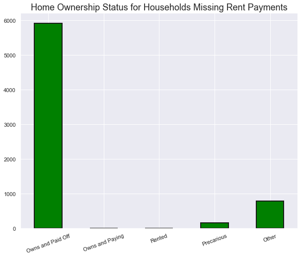
#Looking at the above data it makes sense that when the house is fully paid, there will be no monthly rent payment.
#Lets add 0 for all the null values.
for df in [df_income_train, df_income_test]:
    df['v2a1'].fillna(value=0, inplace=True)

df_income_train[['v2a1']].isnull().sum()
v2a1    0
dtype: int64
# 2. Lets look at v18q1 (total nulls: 7342) : number of tablets household owns
# why the null values, Lets look at few rows with nulls in v18q1
# Columns related to  number of tablets household owns
# v18q, owns a tablet
# Since this is a household variable, it only makes sense to look at it on a household level,
# so we'll only select the rows for the head of household.

# Heads of household
heads = df_income_train.loc[df_income_train['parentesco1'] == 1].copy()
heads.groupby('v18q')['v18q1'].apply(lambda x: x.isnull().sum())
v18q
0    2318
1       0
Name: v18q1, dtype: int64
plt.figure(figsize = (8, 6))
col='v18q1'
df_income_train[col].value_counts().sort_index().plot.bar(color = 'blue',
                                             edgecolor = 'k',
                                             linewidth = 2)
plt.xlabel(f'{col}'); plt.title(f'{col} Value Counts'); plt.ylabel('Count')
plt.show();
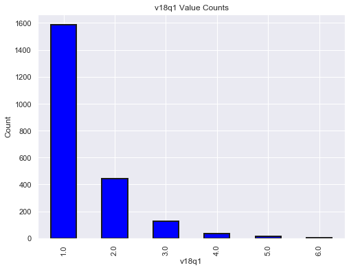
#Looking at the above data it makes sense that when owns a tablet column is 0, there will be no number of tablets household owns.
#Lets add 0 for all the null values.
for df in [df_income_train, df_income_test]:
    df['v18q1'].fillna(value=0, inplace=True)

df_income_train[['v18q1']].isnull().sum()
v18q1    0
dtype: int64
# 3. Lets look at rez_esc    (total nulls: 7928) : Years behind in school
# why the null values, Lets look at few rows with nulls in rez_esc
# Columns related to Years behind in school
# Age in years

# Lets look at the data with not null values first.
df_income_train[df_income_train['rez_esc'].notnull()]['age'].describe()
count    1629.000000
mean       12.258441
std         3.218325
min         7.000000
25%         9.000000
50%        12.000000
75%        15.000000
max        17.000000
Name: age, dtype: float64
#From the above , we see that when min age is 7 and max age is 17 for Years, then the 'behind in school' column has a value.
#Lets confirm
df_income_train.loc[df_income_train['rez_esc'].isnull()]['age'].describe()
count    7928.000000
mean       38.833249
std        20.989486
min         0.000000
25%        24.000000
50%        38.000000
75%        54.000000
max        97.000000
Name: age, dtype: float64
df_income_train.loc[(df_income_train['rez_esc'].isnull() & ((df_income_train['age'] > 7) & (df_income_train['age'] < 17)))]['age'].describe()
#There is one value that has Null for the 'behind in school' column with age between 7 and 17
count     1.0
mean     10.0
std       NaN
min      10.0
25%      10.0
50%      10.0
75%      10.0
max      10.0
Name: age, dtype: float64
df_income_train[(df_income_train['age'] ==10) & df_income_train['rez_esc'].isnull()].head()
df_income_train[(df_income_train['Id'] =='ID_f012e4242')].head()
#there is only one member in household for the member with age 10 and who is 'behind in school'. This explains why the member is
#behind in school.
| Id | v2a1 | hacdor | rooms | hacapo | v14a | refrig | v18q | v18q1 | r4h1 | ... | SQBescolari | SQBage | SQBhogar_total | SQBedjefe | SQBhogar_nin | SQBovercrowding | SQBdependency | SQBmeaned | agesq | Target | |
|---|---|---|---|---|---|---|---|---|---|---|---|---|---|---|---|---|---|---|---|---|---|
| 2514 | ID_f012e4242 | 160000.0 | 0 | 6 | 0 | 1 | 1 | 1 | 1.0 | 0 | ... | 0 | 100 | 9 | 121 | 1 | 2.25 | 0.25 | 182.25 | 100 | 4 |
1 rows × 143 columns
#from above we see that  the 'behind in school' column has null values
# Lets use the above to fix the data
for df in [df_income_train, df_income_test]:
    df['rez_esc'].fillna(value=0, inplace=True)
df_income_train[['rez_esc']].isnull().sum()
rez_esc    0
dtype: int64
#Lets look at meaneduc   (total nulls: 5) : average years of education for adults (18+)
# why the null values, Lets look at few rows with nulls in meaneduc
# Columns related to average years of education for adults (18+)
# edjefe, years of education of male head of household, based on the interaction of escolari (years of education),
#    head of household and gender, yes=1 and no=0
# edjefa, years of education of female head of household, based on the interaction of escolari (years of education),
#    head of household and gender, yes=1 and no=0
# instlevel1, =1 no level of education
# instlevel2, =1 incomplete primary
data = df_income_train[df_income_train['meaneduc'].isnull()].head()

columns=['edjefe','edjefa','instlevel1','instlevel2']
data[columns][data[columns]['instlevel1']>0].describe()
| edjefe | edjefa | instlevel1 | instlevel2 | |
|---|---|---|---|---|
| count | 0.0 | 0.0 | 0.0 | 0.0 |
| mean | NaN | NaN | NaN | NaN |
| std | NaN | NaN | NaN | NaN |
| min | NaN | NaN | NaN | NaN |
| 25% | NaN | NaN | NaN | NaN |
| 50% | NaN | NaN | NaN | NaN |
| 75% | NaN | NaN | NaN | NaN |
| max | NaN | NaN | NaN | NaN |
#from the above, we find that meaneduc is null when no level of education is 0
#Lets fix the data
for df in [df_income_train, df_income_test]:
    df['meaneduc'].fillna(value=0, inplace=True)
df_income_train[['meaneduc']].isnull().sum()
meaneduc    0
dtype: int64
#Lets look at SQBmeaned  (total nulls: 5) : square of the mean years of education of adults (>=18) in the household 142
# why the null values, Lets look at few rows with nulls in SQBmeaned
# Columns related to average years of education for adults (18+)
# edjefe, years of education of male head of household, based on the interaction of escolari (years of education),
#    head of household and gender, yes=1 and no=0
# edjefa, years of education of female head of household, based on the interaction of escolari (years of education),
#    head of household and gender, yes=1 and no=0
# instlevel1, =1 no level of education
# instlevel2, =1 incomplete primary
data = df_income_train[df_income_train['SQBmeaned'].isnull()].head()

columns=['edjefe','edjefa','instlevel1','instlevel2']
data[columns][data[columns]['instlevel1']>0].describe()
| edjefe | edjefa | instlevel1 | instlevel2 | |
|---|---|---|---|---|
| count | 0.0 | 0.0 | 0.0 | 0.0 |
| mean | NaN | NaN | NaN | NaN |
| std | NaN | NaN | NaN | NaN |
| min | NaN | NaN | NaN | NaN |
| 25% | NaN | NaN | NaN | NaN |
| 50% | NaN | NaN | NaN | NaN |
| 75% | NaN | NaN | NaN | NaN |
| max | NaN | NaN | NaN | NaN |
#from the above, we find that SQBmeaned is null when no level of education is 0
#Lets fix the data
for df in [df_income_train, df_income_test]:
    df['SQBmeaned'].fillna(value=0, inplace=True)
df_income_train[['SQBmeaned']].isnull().sum()
SQBmeaned    0
dtype: int64
#Lets look at the overall data
null_counts = df_income_train.isnull().sum()
null_counts[null_counts > 0].sort_values(ascending=False)
Series([], dtype: int64)
3.3 Lets look at the target column
Lets see if records belonging to same household has same target/score.
# Groupby the household and figure out the number of unique values
all_equal = df_income_train.groupby('idhogar')['Target'].apply(lambda x: x.nunique() == 1)

# Households where targets are not all equal
not_equal = all_equal[all_equal != True]
print('There are {} households where the family members do not all have the same target.'.format(len(not_equal)))
There are 85 households where the family members do not all have the same target.
#Lets check one household
df_income_train[df_income_train['idhogar'] == not_equal.index[0]][['idhogar', 'parentesco1', 'Target']]
| idhogar | parentesco1 | Target | |
|---|---|---|---|
| 7651 | 0172ab1d9 | 0 | 3 |
| 7652 | 0172ab1d9 | 0 | 2 |
| 7653 | 0172ab1d9 | 0 | 3 |
| 7654 | 0172ab1d9 | 1 | 3 |
| 7655 | 0172ab1d9 | 0 | 2 |
#Lets use Target value of the parent record (head of the household) and update rest. But before that lets check
# if all families has a head.

households_head = df_income_train.groupby('idhogar')['parentesco1'].sum()

# Find households without a head
households_no_head = df_income_train.loc[df_income_train['idhogar'].isin(households_head[households_head == 0].index), :]

print('There are {} households without a head.'.format(households_no_head['idhogar'].nunique()))
There are 15 households without a head.
# Find households without a head and where Target value are different
households_no_head_equal = households_no_head.groupby('idhogar')['Target'].apply(lambda x: x.nunique() == 1)
print('{} Households with no head have different Target value.'.format(sum(households_no_head_equal == False)))
0 Households with no head have different Target value.
#Lets fix the data
#Set poverty level of the members and the head of the house within a family.
# Iterate through each household
for household in not_equal.index:
    # Find the correct label (for the head of household)
    true_target = int(df_income_train[(df_income_train['idhogar'] == household) & (df_income_train['parentesco1'] == 1.0)]['Target'])

    # Set the correct label for all members in the household
    df_income_train.loc[df_income_train['idhogar'] == household, 'Target'] = true_target


# Groupby the household and figure out the number of unique values
all_equal = df_income_train.groupby('idhogar')['Target'].apply(lambda x: x.nunique() == 1)

# Households where targets are not all equal
not_equal = all_equal[all_equal != True]
print('There are {} households where the family members do not all have the same target.'.format(len(not_equal)))
There are 0 households where the family members do not all have the same target.
3.3 Lets check for any bias in the dataset
#Lets look at the dataset and plot head of household and Target
# 1 = extreme poverty 2 = moderate poverty 3 = vulnerable households 4 = non vulnerable households
target_counts = heads['Target'].value_counts().sort_index()
target_counts
1     222
2     442
3     355
4    1954
Name: Target, dtype: int64
target_counts.plot.bar(figsize = (8, 6),linewidth = 2,edgecolor = 'k',title="Target vs Total_Count")
<matplotlib.axes._subplots.AxesSubplot at 0x1ac071a8cf8>
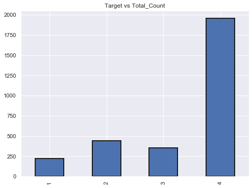
# extreme poverty is the smallest count in the train dataset. The dataset is biased.
3.4 Lets look at the Squared Variables
‘SQBescolari’
‘SQBage’
‘SQBhogar_total’
‘SQBedjefe’
‘SQBhogar_nin’
‘SQBovercrowding’
‘SQBdependency’
‘SQBmeaned’
‘agesq’
#Lets remove them
print(df_income_train.shape)
cols=['SQBescolari', 'SQBage', 'SQBhogar_total', 'SQBedjefe',
        'SQBhogar_nin', 'SQBovercrowding', 'SQBdependency', 'SQBmeaned', 'agesq']


for df in [df_income_train, df_income_test]:
    df.drop(columns = cols,inplace=True)

print(df_income_train.shape)
(9557, 143)
(9557, 134)
id_ = ['Id', 'idhogar', 'Target']

ind_bool = ['v18q', 'dis', 'male', 'female', 'estadocivil1', 'estadocivil2', 'estadocivil3',
            'estadocivil4', 'estadocivil5', 'estadocivil6', 'estadocivil7',
            'parentesco1', 'parentesco2',  'parentesco3', 'parentesco4', 'parentesco5',
            'parentesco6', 'parentesco7', 'parentesco8',  'parentesco9', 'parentesco10',
            'parentesco11', 'parentesco12', 'instlevel1', 'instlevel2', 'instlevel3',
            'instlevel4', 'instlevel5', 'instlevel6', 'instlevel7', 'instlevel8',
            'instlevel9', 'mobilephone']

ind_ordered = ['rez_esc', 'escolari', 'age']

hh_bool = ['hacdor', 'hacapo', 'v14a', 'refrig', 'paredblolad', 'paredzocalo',
           'paredpreb','pisocemento', 'pareddes', 'paredmad',
           'paredzinc', 'paredfibras', 'paredother', 'pisomoscer', 'pisoother',
           'pisonatur', 'pisonotiene', 'pisomadera',
           'techozinc', 'techoentrepiso', 'techocane', 'techootro', 'cielorazo',
           'abastaguadentro', 'abastaguafuera', 'abastaguano',
            'public', 'planpri', 'noelec', 'coopele', 'sanitario1',
           'sanitario2', 'sanitario3', 'sanitario5',   'sanitario6',
           'energcocinar1', 'energcocinar2', 'energcocinar3', 'energcocinar4',
           'elimbasu1', 'elimbasu2', 'elimbasu3', 'elimbasu4',
           'elimbasu5', 'elimbasu6', 'epared1', 'epared2', 'epared3',
           'etecho1', 'etecho2', 'etecho3', 'eviv1', 'eviv2', 'eviv3',
           'tipovivi1', 'tipovivi2', 'tipovivi3', 'tipovivi4', 'tipovivi5',
           'computer', 'television', 'lugar1', 'lugar2', 'lugar3',
           'lugar4', 'lugar5', 'lugar6', 'area1', 'area2']

hh_ordered = [ 'rooms', 'r4h1', 'r4h2', 'r4h3', 'r4m1','r4m2','r4m3', 'r4t1',  'r4t2',
              'r4t3', 'v18q1', 'tamhog','tamviv','hhsize','hogar_nin',
              'hogar_adul','hogar_mayor','hogar_total',  'bedrooms', 'qmobilephone']

hh_cont = ['v2a1', 'dependency', 'edjefe', 'edjefa', 'meaneduc', 'overcrowding']
#Check for redundant household variables
heads = df_income_train.loc[df_income_train['parentesco1'] == 1, :]
heads = heads[id_ + hh_bool + hh_cont + hh_ordered]
heads.shape
(2973, 98)
# Create correlation matrix
corr_matrix = heads.corr()

# Select upper triangle of correlation matrix
upper = corr_matrix.where(np.triu(np.ones(corr_matrix.shape), k=1).astype(np.bool))

# Find index of feature columns with correlation greater than 0.95
to_drop = [column for column in upper.columns if any(abs(upper[column]) > 0.95)]

to_drop
['coopele', 'area2', 'tamhog', 'hhsize', 'hogar_total']
corr_matrix.loc[corr_matrix['tamhog'].abs() > 0.9, corr_matrix['tamhog'].abs() > 0.9]
| r4t3 | tamhog | tamviv | hhsize | hogar_total | |
|---|---|---|---|---|---|
| r4t3 | 1.000000 | 0.996884 | 0.929237 | 0.996884 | 0.996884 |
| tamhog | 0.996884 | 1.000000 | 0.926667 | 1.000000 | 1.000000 |
| tamviv | 0.929237 | 0.926667 | 1.000000 | 0.926667 | 0.926667 |
| hhsize | 0.996884 | 1.000000 | 0.926667 | 1.000000 | 1.000000 |
| hogar_total | 0.996884 | 1.000000 | 0.926667 | 1.000000 | 1.000000 |
sns.heatmap(corr_matrix.loc[corr_matrix['tamhog'].abs() > 0.9, corr_matrix['tamhog'].abs() > 0.9],
            annot=True, cmap = plt.cm.Accent_r, fmt='.3f');
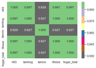
# There are several variables here having to do with the size of the house:
# r4t3, Total persons in the household
# tamhog, size of the household
# tamviv, number of persons living in the household
# hhsize, household size
# hogar_total, # of total individuals in the household
# These variables are all highly correlated with one another.
cols=['tamhog', 'hogar_total', 'r4t3']
for df in [df_income_train, df_income_test]:
    df.drop(columns = cols,inplace=True)

df_income_train.shape
(9557, 131)
#Check for redundant Individual variables
ind = df_income_train[id_ + ind_bool + ind_ordered]
ind.shape
(9557, 39)
# Create correlation matrix
corr_matrix = ind.corr()

# Select upper triangle of correlation matrix
upper = corr_matrix.where(np.triu(np.ones(corr_matrix.shape), k=1).astype(np.bool))

# Find index of feature columns with correlation greater than 0.95
to_drop = [column for column in upper.columns if any(abs(upper[column]) > 0.95)]

to_drop
['female']
# This is simply the opposite of male! We can remove the male flag.
for df in [df_income_train, df_income_test]:
    df.drop(columns = 'male',inplace=True)

df_income_train.shape
(9557, 130)
#lets check area1 and area2 also
# area1, =1 zona urbana
# area2, =2 zona rural
#area2 redundant because we have a column indicating if the house is in a urban zone

for df in [df_income_train, df_income_test]:
    df.drop(columns = 'area2',inplace=True)

df_income_train.shape
(9557, 129)
#Finally lets delete 'Id', 'idhogar'
cols=['Id','idhogar']
for df in [df_income_train, df_income_test]:
    df.drop(columns = cols,inplace=True)

df_income_train.shape
(9557, 127)
Step 4: Predict the accuracy using random forest classifier.
x_features=df_income_train.iloc[:,0:-1]
y_features=df_income_train.iloc[:,-1]
print(x_features.shape)
print(y_features.shape)
(9557, 126)
(9557,)
from sklearn.ensemble import RandomForestClassifier
from sklearn.model_selection import train_test_split
from sklearn.metrics import accuracy_score,confusion_matrix,f1_score,classification_report

x_train,x_test,y_train,y_test=train_test_split(x_features,y_features,test_size=0.2,random_state=1)
rmclassifier = RandomForestClassifier()
rmclassifier.fit(x_train,y_train)
RandomForestClassifier(bootstrap=True, class_weight=None, criterion='gini',
                       max_depth=None, max_features='auto', max_leaf_nodes=None,
                       min_impurity_decrease=0.0, min_impurity_split=None,
                       min_samples_leaf=1, min_samples_split=2,
                       min_weight_fraction_leaf=0.0, n_estimators=10,
                       n_jobs=None, oob_score=False, random_state=None,
                       verbose=0, warm_start=False)
y_predict = rmclassifier.predict(x_test)
print(accuracy_score(y_test,y_predict))
print(confusion_matrix(y_test,y_predict))
print(classification_report(y_test,y_predict))
0.9267782426778243
[[ 124    7    2   24]
 [   1  276    4   36]
 [   0   12  183   38]
 [   2    9    5 1189]]
              precision    recall  f1-score   support

           1       0.98      0.79      0.87       157
           2       0.91      0.87      0.89       317
           3       0.94      0.79      0.86       233
           4       0.92      0.99      0.95      1205

    accuracy                           0.93      1912
   macro avg       0.94      0.86      0.89      1912
weighted avg       0.93      0.93      0.92      1912
y_predict_testdata = rmclassifier.predict(df_income_test)
y_predict_testdata
array([4, 4, 4, ..., 4, 4, 2], dtype=int64)
Step 6: Check the accuracy using random forest with cross validation.
from sklearn.model_selection import KFold,cross_val_score
6.1 Checking the score using default 10 trees
seed=7
kfold=KFold(n_splits=5,random_state=seed,shuffle=True)

rmclassifier=RandomForestClassifier(random_state=10,n_jobs = -1)
print(cross_val_score(rmclassifier,x_features,y_features,cv=kfold,scoring='accuracy'))
results=cross_val_score(rmclassifier,x_features,y_features,cv=kfold,scoring='accuracy')
print(results.mean()*100)
[0.93514644 0.93043933 0.92569335 0.9314495  0.9314495 ]
93.08356268159017
6.2 Checking the score using 100 trees
num_trees= 100

rmclassifier=RandomForestClassifier(n_estimators=100, random_state=10,n_jobs = -1)
print(cross_val_score(rmclassifier,x_features,y_features,cv=kfold,scoring='accuracy'))
results=cross_val_score(rmclassifier,x_features,y_features,cv=kfold,scoring='accuracy')
print(results.mean()*100)
[0.94246862 0.94979079 0.94557823 0.94243851 0.94976452]
94.60081361157272
y_predict_testdata = rmclassifier.predict(df_income_test)
y_predict_testdata
array([4, 4, 4, ..., 4, 4, 4], dtype=int64)
Looking at the accuracy score, RandomForestClassifier with cross validation has the highest accuracy score of 94.60%
To get a better sense of what is going on inside the RandomForestClassifier model, lets visualize how our model uses the different features and which features have greater effect.
rmclassifier.fit(x_features,y_features)
labels = list(x_features)
feature_importances = pd.DataFrame({'feature': labels, 'importance': rmclassifier.feature_importances_})
feature_importances=feature_importances[feature_importances.importance>0.015]
feature_importances.head()
| feature | importance | |
|---|---|---|
| 0 | v2a1 | 0.018653 |
| 2 | rooms | 0.025719 |
| 9 | r4h2 | 0.020706 |
| 10 | r4h3 | 0.019808 |
| 11 | r4m1 | 0.015271 |
feature_importances.sort_values(by=['importance'], ascending=True, inplace=True)
feature_importances['positive'] = feature_importances['importance'] > 0
feature_importances.set_index('feature',inplace=True)
feature_importances.head()

feature_importances.importance.plot(kind='barh', figsize=(11, 6),color = feature_importances.positive.map({True: 'blue', False: 'red'}))
plt.xlabel('Importance')
Text(0.5, 0, 'Importance')
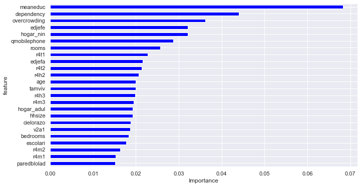
From the above figure, meaneduc,dependency,overcrowding has significant influence on the model.