
Strength Of High Performance Concrete
Overview:
For this exercise, we will utilize data on the compressive strength of concrete donated to the UCI Machine Learning Data Repository (http://archive.ics.uci.edu/ml) by I-Cheng Yeh.
For more information on Yeh’s approach to this learning task, refer to: Yeh IC. Modeling of strength of high performance concrete using artificial neural networks. Cement and Concrete Research. 1998; 28:1797-1808. According to the website, the concrete dataset contains 1,030 examples of concrete with eight features describing the components used in the mixture.
These features are thought to be related to the final compressive strength and they include the amount (in kilograms per cubic meter) of cement, slag, ash, water, superplasticizer, coarse aggregate, and fine aggregate used in the product in addition to the aging time (measured in days).
Problem Statement Scenario:
Determine strenth of concrete in terms of 8 features.
Following actions should be performed:
Apply various Regression Algorithm and compare Rmse and R2. Tune the base mode.
Preprocess Data:
1.1 Check data
#import necessary libraries
import pandas as pd
import numpy as np

import matplotlib.pyplot as plt
%matplotlib inline
import seaborn as sns
sns.set()

import warnings
warnings.filterwarnings('ignore')

from math import sqrt
from sklearn.linear_model import LinearRegression,Lasso,Ridge,ElasticNet
from sklearn.metrics import mean_squared_error ,r2_score,adjusted_rand_score,mean_absolute_error
from sklearn.model_selection import train_test_split, KFold,cross_val_score
from sklearn.preprocessing import StandardScaler
from sklearn.ensemble import RandomForestRegressor,GradientBoostingRegressor
from sklearn.tree import DecisionTreeRegressor
import pickle
df=pd.read_csv("Dataset/concrete.csv")
df.shape
(1030, 9)
#Check first 5 records
df.head()
| cement | slag | ash | water | superplastic | coarseagg | fineagg | age | strength | |
|---|---|---|---|---|---|---|---|---|---|
| 0 | 141.3 | 212.0 | 0.0 | 203.5 | 0.0 | 971.8 | 748.5 | 28 | 29.89 |
| 1 | 168.9 | 42.2 | 124.3 | 158.3 | 10.8 | 1080.8 | 796.2 | 14 | 23.51 |
| 2 | 250.0 | 0.0 | 95.7 | 187.4 | 5.5 | 956.9 | 861.2 | 28 | 29.22 |
| 3 | 266.0 | 114.0 | 0.0 | 228.0 | 0.0 | 932.0 | 670.0 | 28 | 45.85 |
| 4 | 154.8 | 183.4 | 0.0 | 193.3 | 9.1 | 1047.4 | 696.7 | 28 | 18.29 |
#Check for null values
df.isnull().sum()
cement          0
slag            0
ash             0
water           0
superplastic    0
coarseagg       0
fineagg         0
age             0
strength        0
dtype: int64
#check if there is any categorical feature
df.dtypes
cement          float64
slag            float64
ash             float64
water           float64
superplastic    float64
coarseagg       float64
fineagg         float64
age               int64
strength        float64
dtype: object
1.2 Lets normalize the dataset
# Get column names first
columnname = df.columns
# Create the Scaler object
scaler = StandardScaler()
# Fit your data on the scaler object
scaled_df = scaler.fit_transform(df)
scaled_df = pd.DataFrame(scaled_df, columns=columnname)
scaled_df.head()
| cement | slag | ash | water | superplastic | coarseagg | fineagg | age | strength | |
|---|---|---|---|---|---|---|---|---|---|
| 0 | -1.339017 | 1.601441 | -0.847144 | 1.027590 | -1.039143 | -0.014398 | -0.312970 | -0.279733 | -0.355018 |
| 1 | -1.074790 | -0.367541 | 1.096078 | -1.090116 | 0.769617 | 1.388141 | 0.282260 | -0.501465 | -0.737108 |
| 2 | -0.298384 | -0.856888 | 0.648965 | 0.273274 | -0.118015 | -0.206121 | 1.093371 | -0.279733 | -0.395144 |
| 3 | -0.145209 | 0.465044 | -0.847144 | 2.175461 | -1.039143 | -0.526517 | -1.292542 | -0.279733 | 0.600806 |
| 4 | -1.209776 | 1.269798 | -0.847144 | 0.549700 | 0.484905 | 0.958372 | -0.959363 | -0.279733 | -1.049727 |
1.3 Check for correlation
corr = df.corr()
print(corr)
plt.figure(figsize=(15,10))
sns.heatmap(corr,
        xticklabels=corr.columns,
        yticklabels=corr.columns)
                cement      slag       ash     water  superplastic  coarseagg  \
cement        1.000000 -0.275216 -0.397467 -0.081587      0.092386  -0.109349
slag         -0.275216  1.000000 -0.323580  0.107252      0.043270  -0.283999
ash          -0.397467 -0.323580  1.000000 -0.256984      0.377503  -0.009961
water        -0.081587  0.107252 -0.256984  1.000000     -0.657533  -0.182294
superplastic  0.092386  0.043270  0.377503 -0.657533      1.000000  -0.265999
coarseagg    -0.109349 -0.283999 -0.009961 -0.182294     -0.265999   1.000000
fineagg      -0.222718 -0.281603  0.079108 -0.450661      0.222691  -0.178481
age           0.081946 -0.044246 -0.154371  0.277618     -0.192700  -0.003016
strength      0.497832  0.134829 -0.105755 -0.289633      0.366079  -0.164935

               fineagg       age  strength
cement       -0.222718  0.081946  0.497832
slag         -0.281603 -0.044246  0.134829
ash           0.079108 -0.154371 -0.105755
water        -0.450661  0.277618 -0.289633
superplastic  0.222691 -0.192700  0.366079
coarseagg    -0.178481 -0.003016 -0.164935
fineagg       1.000000 -0.156095 -0.167241
age          -0.156095  1.000000  0.328873
strength     -0.167241  0.328873  1.000000


<matplotlib.axes._subplots.AxesSubplot at 0x1c942fb3c88>
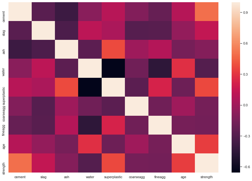
From the above heatmap , we see that there is high correlation between Strenth and Cement,age
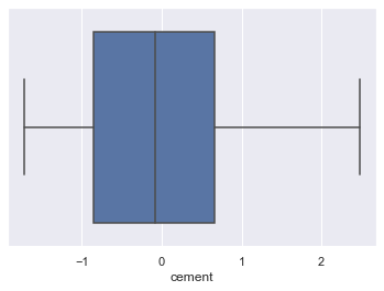
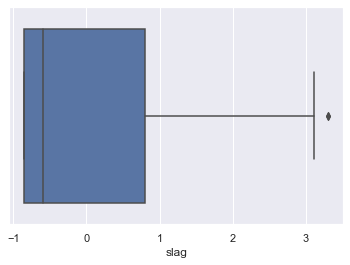
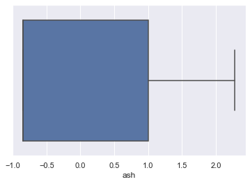
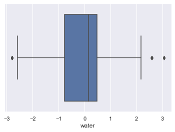
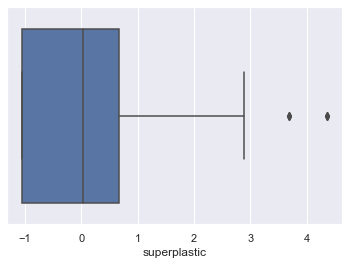
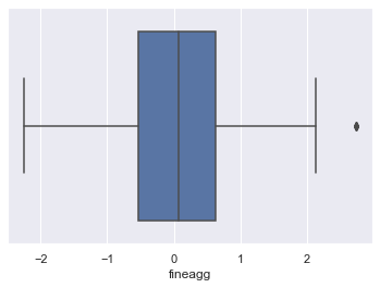
1.4 Check for Outliers and remove them
for column in scaled_df:
    plt.figure()
    sns.boxplot(x=scaled_df[column])

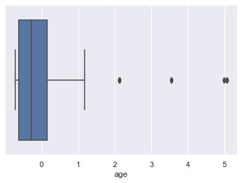
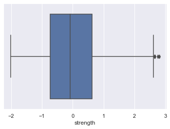
Lets look at age outliers
filter =scaled_df['age'].values>1.5
df_outlier_slag=scaled_df[filter]
df_outlier_slag.shape
(59, 9)
We found that there are 59 rows that have higher value then rest. This is a large number of records out of 1030. If we remove the outliers we will lose lot of information. Lets keep them.
2. Split data into Train and Test datasets
x_features=scaled_df.drop(['strength'],axis=1)
y_features=scaled_df['strength']

x_train,x_test,y_train,y_test = train_test_split(x_features,y_features,test_size=0.2,random_state=1)

print(x_train.shape)
print(x_test.shape)
print(y_train.shape)
print(y_test.shape)
(824, 8)
(206, 8)
(824,)
(206,)
3. Lets apply different models and check R2 and RMSE values
Model = []
RMSE = []
R_sq = []
cv = KFold(5, random_state = 1)

#Creating a Function to append the cross validation scores of the algorithms
def input_scores(name, model, x, y):
    Model.append(name)
    RMSE.append(np.sqrt((-1) * cross_val_score(model, x, y, cv=cv,
                                               scoring='neg_mean_squared_error').mean()))
    R_sq.append(cross_val_score(model, x, y, cv=cv, scoring='r2').mean())
from sklearn.linear_model import LinearRegression, Ridge, Lasso
from sklearn.neighbors import KNeighborsRegressor
from sklearn.tree import DecisionTreeRegressor
from sklearn.ensemble import (RandomForestRegressor, GradientBoostingRegressor,
                              AdaBoostRegressor)

names = ['Linear Regression', 'Ridge Regression', 'Lasso Regression',
         'K Neighbors Regressor', 'Decision Tree Regressor',
         'Random Forest Regressor', 'Gradient Boosting Regressor',
         'Adaboost Regressor']
models = [LinearRegression(), Ridge(), Lasso(),
          KNeighborsRegressor(), DecisionTreeRegressor(),
          RandomForestRegressor(), GradientBoostingRegressor(),
          AdaBoostRegressor()]

#Running all algorithms
for name, model in zip(names, models):
    input_scores(name, model, x_train, y_train)
model_results = pd.DataFrame({'Model': Model,
                           'RMSE': RMSE,
                           'R2': R_sq})
print("FOLLOWING ARE THE TRAINING SCORES: ")
model_results
FOLLOWING ARE THE TRAINING SCORES:
| Model | RMSE | R2 | |
|---|---|---|---|
| 0 | Linear Regression | 0.628006 | 0.599298 |
| 1 | Ridge Regression | 0.628072 | 0.599195 |
| 2 | Lasso Regression | 0.993427 | -0.003958 |
| 3 | K Neighbors Regressor | 0.552880 | 0.688894 |
| 4 | Decision Tree Regressor | 0.422913 | 0.825952 |
| 5 | Random Forest Regressor | 0.329487 | 0.885011 |
| 6 | Gradient Boosting Regressor | 0.318054 | 0.897072 |
| 7 | Adaboost Regressor | 0.470504 | 0.777779 |
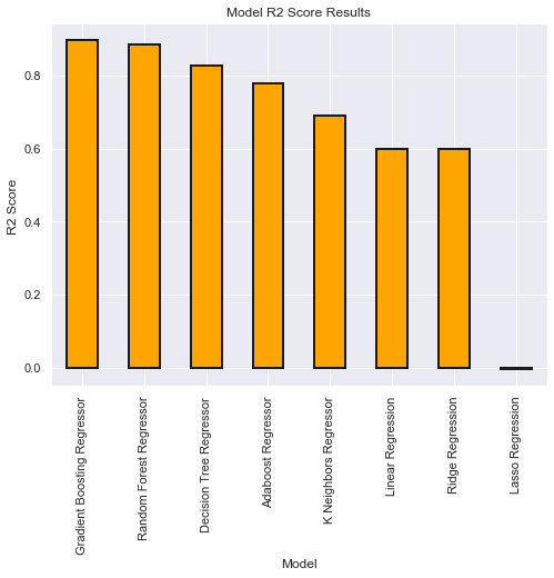
model_results=model_results.sort_values(by='R2',ascending=False)
model_results.set_index('Model', inplace = True)
model_results['R2'].plot.bar(color = 'orange', figsize = (8, 6),
                                 edgecolor = 'k', linewidth = 2)
plt.title('Model R2 Score Results');
plt.ylabel('R2 Score ');
model_results.reset_index(inplace = True)
model_results=model_results.sort_values(by='RMSE',ascending=False)
model_results.set_index('Model', inplace = True)
model_results['RMSE'].plot.bar(color = 'blue', figsize = (8, 6),
                                 edgecolor = 'k', linewidth = 2)
plt.title('Model RMSE Score Results');
plt.ylabel('Model');
model_results.reset_index(inplace = True)
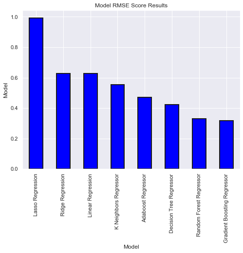
We found that the best performingand low error model is Gardient Boosting Regressor. Lets tune the model.
GradientBoostingRegressor()
GradientBoostingRegressor(alpha=0.9, criterion='friedman_mse', init=None,
                          learning_rate=0.1, loss='ls', max_depth=3,
                          max_features=None, max_leaf_nodes=None,
                          min_impurity_decrease=0.0, min_impurity_split=None,
                          min_samples_leaf=1, min_samples_split=2,
                          min_weight_fraction_leaf=0.0, n_estimators=100,
                          n_iter_no_change=None, presort='auto',
                          random_state=None, subsample=1.0, tol=0.0001,
                          validation_fraction=0.1, verbose=0, warm_start=False)
#tuning for number of trees
from sklearn.model_selection import GridSearchCV
param_grid = {'n_estimators':range(20,1001,10),
              'max_depth':[10], #range(5,16,2),
              'min_samples_split':[100], #range(200,1001,200),
              'learning_rate':[0.2]}
clf = GridSearchCV(GradientBoostingRegressor(random_state=1),
                   param_grid = param_grid, scoring='r2',
                   cv=cv).fit(x_train, y_train)
print(clf.best_estimator_)
print("R Squared:",clf.best_score_)
GradientBoostingRegressor(alpha=0.9, criterion='friedman_mse', init=None,
                          learning_rate=0.2, loss='ls', max_depth=10,
                          max_features=None, max_leaf_nodes=None,
                          min_impurity_decrease=0.0, min_impurity_split=None,
                          min_samples_leaf=1, min_samples_split=100,
                          min_weight_fraction_leaf=0.0, n_estimators=210,
                          n_iter_no_change=None, presort='auto', random_state=1,
                          subsample=1.0, tol=0.0001, validation_fraction=0.1,
                          verbose=0, warm_start=False)
R Squared: 0.9283739412935808
#tuning the tree specific parameters
param_grid = {'n_estimators': [230],
              'max_depth': range(10,31,2),
              'min_samples_split': range(50,501,10),
              'learning_rate':[0.2]}
clf = GridSearchCV(GradientBoostingRegressor(random_state=1),
                   param_grid = param_grid, scoring='r2',
                   cv=cv).fit(x_train, y_train)
print(clf.best_estimator_)
print("R Squared:",clf.best_score_)
GradientBoostingRegressor(alpha=0.9, criterion='friedman_mse', init=None,
                          learning_rate=0.2, loss='ls', max_depth=24,
                          max_features=None, max_leaf_nodes=None,
                          min_impurity_decrease=0.0, min_impurity_split=None,
                          min_samples_leaf=1, min_samples_split=200,
                          min_weight_fraction_leaf=0.0, n_estimators=230,
                          n_iter_no_change=None, presort='auto', random_state=1,
                          subsample=1.0, tol=0.0001, validation_fraction=0.1,
                          verbose=0, warm_start=False)
R Squared: 0.934160327594603
#now increasing number of trees and decreasing learning rate proportionally
clf = GradientBoostingRegressor(random_state=1, max_depth=20,
                                min_samples_split=170, n_estimators=230*2,
                                learning_rate=0.2/2)
print("R Squared:",cross_val_score(clf, x_train, y_train, cv=cv, scoring='r2').mean())
R Squared: 0.9339536875739721
Since score improved, the best model is GradientBoostingRegressor with learning_rate= 0.2/2, max_depth= 20, min_samples_split= 170, n_estimators= 230*2
min_samples_split = 170
n_estimators= 230*2

#applying this model on test data
#x_test = pd.DataFrame(x_test,
#                             columns = x_test.columns)
clf = GradientBoostingRegressor(learning_rate=0.2/2, max_depth=20,
                                min_samples_split=170, n_estimators=230*2,
                                random_state=1).fit(x_train, y_train)
print("Test RMSE: ", np.sqrt(mean_squared_error(y_test, clf.predict(x_test_scaled))))
print("Test R^2: ", r2_score(y_test, clf.predict(x_test_scaled)))
Test RMSE:  0.23046182859820957
Test R^2:  0.9497116031799179
# save the model to disk
filename = 'model/finalized_model.pkl'
pickle.dump(clf, open(filename, 'wb'))